


In image processing it is quite common to use simple statistical descriptions of images and sub-images. The notion of a statistic is intimately connected to the concept of a probability distribution, generally the distribution of signal amplitudes. For a given region--which could conceivably be an entire image--we can define the probability distribution function of the brightnesses in that region and the probability density function of the brightnesses in that region. We will assume in the discussion that follows that we are dealing with a digitized image a[m,n].
 to
+
to
+ , P(a) increases from 0 to 1. P(a) is
monotonic, non-decreasing in a and thus dP/da >= 0.
 a, given the probability distribution function
P(a), can be expressed as
p(a)
 a where p(a) is the
probability density function:

T.1 Rectangle
|

|

|

|
| picture
1
|
picture
2
|
T.2 Pyramid
|

|

|

|
| picture
1
|
picture
2
|
T.3 Pill Box
|

|

|

|
| picture
1
|
picture
2
|
T.4 Cone
|

|

|

|
| picture
1
|
picture
2
|
T.5 Airy PSF
|

|

|
|
| picture
1
|
picture
2
|
T.6 Gaussian
|

|

|

|
| picture
1
|
picture
2
|
T.7 Peak
|

|

|

|
| picture
1
|
picture
2
|
T.8 Exponential
Decay
|

|

|

|
| picture
1
|
picture
2
|

For an image with quantized (integer) brightness amplitudes, the interpretation
of  a is the width of a brightness interval. We assume
constant width intervals. The brightness probability density function is
frequently estimated by counting the number of times that each brightness
occurs in the region to generate a histogram, h[a]. The histogram
can then be normalized so that the total area under the histogram is 1 (eq. ).
Said another way, the p[a] for a region is the normalized count
of the number of pixels,
  , in a region that have
quantized brightness a:

The brightness probability distribution function for the image shown in Figure 4a is shown in Figure 6a. The (unnormalized) brightness histogram of Figure 4a which is proportional to the estimated brightness probability density function is shown in Figure 6b. The height in this histogram corresponds to the number of pixels with a given brightness.
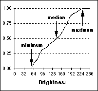
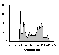
Figure 6: (a) Brightness distribution function of Figure 4a with minimum, median, and maximum indicated. See text for explanation. (b) Brightness histogram of Figure 4a.
Both the distribution function and the histogram as measured from a region are a statistical description of that region. It must be emphasized that both P[a] and p[a] should be viewed as estimates of true distributions when they are computed from a specific region. That is, we view an image and a specific region as one realization of the various random processes involved in the formation of that image and that region. In the same context, the statistics defined below must be viewed as estimates of the underlying parameters.
 pixels within a region (
 ) is given by:

Alternatively, we can use a formulation based upon the (unnormalized)
brightness histogram, h(a) =
 *p(a), with discrete brightness
values a. This gives:

The average brightness, ma, is an estimate of the mean brightness, ua, of the underlying brightness probability distribution.
 )
with
  pixels is called the sample
standard deviation and is given by:
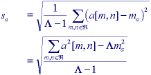
Using the histogram formulation gives:

The standard deviation, sa, is an estimate of
 a of the underlying brightness
probability distribution.


Three special cases are frequently used in digital image processing.
* 0% the minimum value in the region
* 50% the median value in the region
* 100% the maximum value in the region
All three of these values can be determined from Figure 6a.

If the signal is not bounded but has a statistical distribution then two other definitions are known:


where ma and sa are defined above.
The various statistics are given in Table 5 for the image and the region shown in Figure 7.
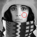
 Figure 7 Table 5 Region is the interior of the circle. Statistics from
Figure 7
A SNR calculation for the entire image based on eq. is not
directly available. The variations in the image brightnesses that lead to the
large value of s (=49.5) are not, in general, due to noise but to the
variation in local information. With the help of the region there is a way to
estimate the SNR. We can use the s (=4.0) and the dynamic range, amax - amin,
for the image (=241-56) to calculate a global SNR (=33.3 dB). The
underlying assumptions are that 1) the signal is approximately constant in that
region and the variation in the region is therefore due to noise, and, 2) that
the noise is the same over the entire image with a standard deviation given by
sn = s
 .
.
