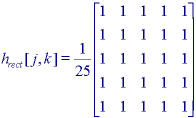
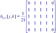
 (a) Rectangular filter (J=K=5) (b) Circular filter
(R=2.5)
 Figure 26: Uniform filters for image smoothing


These algorithms are applied in order to reduce noise and/or to prepare images for further processing such as segmentation. We distinguish between linear and non- linear algorithms where the former are amenable to analysis in the Fourier domain and the latter are not. We also distinguish between implementations based on a rectangular support for the filter and implementations based on a circular support for the filter.
* Uniform filter - The output image is based on a local averaging of the input filter where all of the values within the filter support have the same weight. In the continuous spatial domain (x,y) the PSF and transfer function are given in Table 4-T.1 for the rectangular case and in Table 4-T.3 for the circular (pill box) case. For the discrete spatial domain [m,n] the filter values are the samples of the continuous domain case. Examples for the rectangular case (J=K=5) and the circular case (R=2.5) are shown in Figure 26.

 (a) Rectangular filter (J=K=5) (b) Circular filter
(R=2.5)
 Figure 26: Uniform filters for image smoothing
Note that in both cases the filter is normalized so that  h[j,k] = 1. This is done so that if the input
a[m,n] is a constant then the output image
c[m,n] is the same constant. The justification can be
found in the Fourier transform property described in eq. . As can be seen from
Table 4, both of these filters have transfer functions that have
negative lobes and can, therefore, lead to phase reversal as seen in Figure 23.
The square implementation of the filter is separable and incremental; the
circular implementation is incremental .
* Triangular filter - The output image is based on a local averaging of the input filter where the values within the filter support have differing weights. In general, the filter can be seen as the convolution of two (identical) uniform filters either rectangular or circular and this has direct consequences for the computational complexity . (See Table 13.) In the continuous spatial domain the PSF and transfer function are given in Table 4-T.2 for the rectangular support case and in Table 4-T.4 for the circular (pill box) support case. As seen in Table 4 the transfer functions of these filters do not have negative lobes and thus do not exhibit phase reversal.
Examples for the rectangular support case (J=K=5) and the
circular support case (R=2.5) are shown in Figure 27. The filter is
again normalized so that  h[j,k]=1.
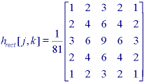
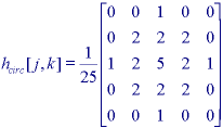
Figure 27: Triangular filters for image smoothing
* Gaussian filter - The use of the Gaussian kernel for smoothing has become extremely popular. This has to do with certain properties of the Gaussian (e.g. the central limit theorem, minimum space-bandwidth product) as well as several application areas such as edge finding and scale space analysis. The PSF and transfer function for the continuous space Gaussian are given in Table 4-T6. The Gaussian filter is separable:

There are four distinct ways to implement the Gaussian:
- Convolution using a finite number of samples (No) of the
Gaussian as the convolution kernel. It is common to choose No
=  3
3
 or
or
 5
5
 .
.

- Repetitive convolution using a uniform filter as the convolution kernel.

The actual implementation (in each dimension) is usually of the form:

This implementation makes use of the approximation afforded by the central
limit theorem. For a desired  with eq. , we use
No =

 although this
severely restricts our choice of
  's to integer values.
- Multiplication in the frequency domain. As the Fourier transform of a
Gaussian is a Gaussian (see Table -T.6), this means that it is
straightforward to prepare a filter ( ,
, ) =
G2D(
 ,
, ) for use with eq. . To
avoid truncation effects in the frequency domain due to the infinite extent of
the Gaussian it is important to choose a
  that is sufficiently
large. Choosing
  > k/
> k/ where k = 3 or 4
will usually be sufficient.
- Use of a recursive filter implementation. A recursive filter has an infinite
impulse response and thus an infinite support. The separable Gaussian filter
can also be implemented by applying the following recipe in each dimension
when  >= 0.5.
 based on the desired goal of the
filtering; ii) Determine the parameter q based on eq. ;
iii) Use eq. to determine the filter coefficients
{b0,b1,b2,b3,B};
iv) Apply the forward difference equation, eq. ; v) Apply the
backward difference equation, eq. ;
The relation between the desired  and q is given by:

The filter coefficients {b0,b1,b2,b3,B} are defined by:
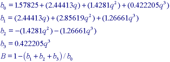
The one-dimensional forward difference equation takes an input row (or column) a[n] and produces an intermediate output result w[n] given by:

The one-dimensional backward difference equation takes the intermediate result w[n] and produces the output c[n] given by:

The forward equation is applied from n = 0 up to n = N - 1 while the backward equation is applied from n = N - 1 down to n = 0.
The relative performance of these various implementation of the Gaussian filter
can be described as follows. Using the root-square error
 between a true, infinite-extent Gaussian, g[n|
 ],
and an approximated Gaussian, h[n], as a measure of accuracy, the
various algorithms described above give the results shown in Figure. 28a. The
relative speed of the various algorithms in shown in Figure 28b.
The root-square error measure is extremely conservative and thus all filters,
with the exception of "Uniform 3x" for large  , are
sufficiently accurate. The recursive implementation is the fastest independent
of
  ; the other implementations can be significantly slower. The
FFT implementation, for example, is 3.1 times slower for N=256 .
Further, the FFT requires that N be a highly composite number.
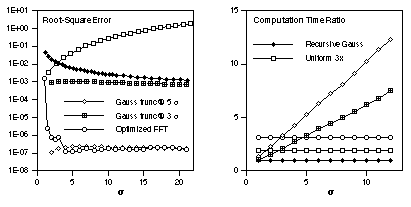
Figure 28: Comparison of various Gaussian algorithms with N=256. The legend is spread across both graphs
* Other - The Fourier domain approach offers the opportunity to
implement a variety of smoothing algorithms. The smoothing filters will then be
lowpass filters. In general it is desirable to use a lowpass
filter that has zero phase so as not to produce phase distortion when filtering
the image. The importance of phase was illustrated in Figures 5 and 23. When
the frequency domain characteristics can be represented in an analytic form,
then this can lead to relatively straightforward implementations of
( ,
, ). Possible candidates include the lowpass
filters "Airy" and "Exponential Decay" found in Table 4-T.5 and Table 4-T.8,
respectively.
* Median filter - The median statistic was described in Section 3.5.2. A median filter is based upon moving a window over an image (as in a convolution) and computing the output pixel as the median value of the brightnesses within the input window. If the window is J x K in size we can order the J*K pixels in brightness value from smallest to largest. If J*K is odd then the median will be the (J*K+1)/2 entry in the list of ordered brightnesses. Note that the value selected will be exactly equal to one of the existing brightnesses so that no roundoff error will be involved if we want to work exclusively with integer brightness values. The algorithm as it is described above has a generic complexity per pixel of O(J*K*log(J*K)). Fortunately, a fast algorithm (due to uang et al. ) exists that reduces the complexity to O(K) assuming J >= K.
A useful variation on the theme of the median filter is the percentile filter. ere the center pixel in the window is replaced not by the 50% (median) brightness value but rather by the p% brightness value where p% ranges from 0% (the minimum filter) to 100% (the maximum filter). Values other then (p=50)% do not, in general, correspond to smoothing filters.
* Kuwahara filter - Edges play an important role in our perception of images (see Figure 15) as well as in the analysis of images. As such it is important to be able to smooth images without disturbing the sharpness and, if possible, the position of edges. A filter that accomplishes this goal is termed an edge-preserving filter and one particular example is the Kuwahara filter . Although this filter can be implemented for a variety of different window shapes, the algorithm will be described for a square window of size J = K = 4L + 1 where L is an integer. The window is partitioned into four regions as shown in Figure 29.
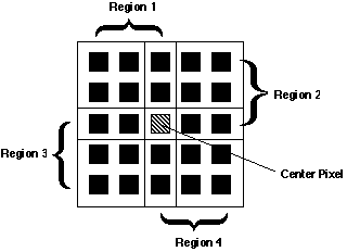
Figure 29: Four, square regions defined for the Kuwahara filter. In this example L=1 and thus J=K=5. Each region is [(J+1)/2] x [(K+1)/2].
In each of the four regions (i=1,2,3,4), the mean brightness, mi in eq. , and the variancei, si2 in eq. , are measured. The output value of the center pixel in the window is the mean value of that region that has the smallest variance.
Algorithm
|
Domain
|
Type
|
Support
|
Separable
/ Incremental
|
Complexity/pixel
|
| Uniform
|
Space
|
Linear
|
Square
|
Y
/ Y
|
O(constant)
|
| Uniform
|
Space
|
Linear
|
Circular
|
N
/ Y
|
O(K)
|
| Triangle
|
Space
|
Linear
|
Square
|
Y
/ N
|
O(constant)
ª
|
| Triangle
|
Space
|
Linear
|
Circular
|
N
/ N
|
O(K)
ª
|
| Gaussian
|
Space
|
Linear
|
 ª
ª
|
Y
/ N
|
O(constant)
ª
|
| Median
|
Space
|
Non-Linear
|
Square
|
N
/ Y
|
O(K)
ª
|
| Kuwahara
|
Space
|
Non-Linear
|
Square
ª
|
N
/ N
|
O(J*
K)
|
| Other
|
Frequency
|
Linear
|
--
|
--
/ --
|
O(logN)
|
Examples of the effect of various smoothing algorithms are shown in Figure 30.
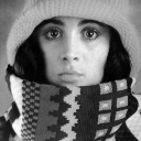


 = 2.5)

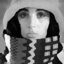 d) Median 5 x 5 e) Kuwahara 5 x 5
Figure 30: Illustration of various linear and non-linear smoothing filters
