


Just as smoothing is a fundamental operation in image processing so is the ability to take one or more spatial derivatives of the image. The fundamental problem is that, according to the mathematical definition of a derivative, this cannot be done. A digitized image is not a continuous function a(x,y) of the spatial variables but rather a discrete function a[m,n] of the integer spatial coordinates. As a result the algorithms we will present can only be seen as approximations to the true spatial derivatives of the original spatially-continuous image.
Further, as we can see from the Fourier property in eq. , taking a derivative multiplies the signal spectrum by either u or v. This means that high frequency noise will be emphasized in the resulting image. The general solution to this problem is to combine the derivative operation with one that suppresses high frequency noise, in short, smoothing in combination with the desired derivative operation.
 to denote the arbitrary angle derivative
filter (matrix), then:

* Gradient filters - It is also possible to generate a vector
derivative description as the gradient,
 a[m,n], of an image:

where
 are unit vectors in the horizontal and vertical direction, respectively. This
leads to two descriptions:

and

The gradient magnitude is sometimes approximated by:

The final results of these calculations depend strongly on the choices of hx and hy. A number of possible choices for (hx, hy) will now be described.
* Basic derivative filters - These filters are specified by:

where "t" denotes matrix transpose. These two filters differ
significantly in their Fourier magnitude and Fourier phase characteristics. For
the frequency range 0 <=  <=
<=  , these are given by:

The second form (ii) gives suppression of high frequency terms
( ~
~  ) while the first form (i) does not. The first
form leads to a phase shift; the second form does not.
* Prewitt gradient filters - These filters are specified by:
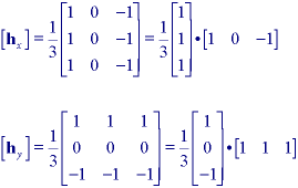
Both hx and hy are separable. Beyond the computational implications are the implications for the analysis of the filter. Each filter takes the derivative in one direction using eq. ii and smoothes in the orthogonal direction using a one-dimensional version of a uniform filter as described in Section 9.4.1.
* Sobel gradient filters - These filters are specified by:
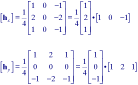
Again, hx and hy are separable. Each filter takes the derivative in one direction using eq. ii and smoothes in the orthogonal direction using a one-dimensional version of a triangular filter as described in Section 9.4.1.
* Alternative gradient filters - The variety of techniques available from one-dimensional signal processing for the design of digital filters offers us powerful tools for designing one-dimensional versions of hx and hy. Using the Parks-McClellan filter design algorithm, for example, we can choose the frequency bands where we want the derivative to be taken and the frequency bands where we want the noise to be suppressed. The algorithm will then produce a real, odd filter with a minimum length that meets the specifications.
As an example, if we want a filter that has derivative characteristics in a
passband (with weight 1.0) in the frequency range 0.0 <=  <= 0.3
 and a stopband (with weight 3.0) in the range 0.32
 <=
<=
 <=
<=  , then the algorithm produces the following
optimized seven sample filter:

The gradient can then be calculated as in eq. .
* Gaussian gradient filters - In modern digital image processing one of the most common techniques is to use a Gaussian filter (see Section 9.4.1) to accomplish the required smoothing and one of the derivatives listed in eq. . Thus, we might first apply the recursive Gaussian in eq. followed by eq. ii to achieve the desired, smoothed derivative filters hx and hy. Further, for computational efficiency, we can combine these two steps as:

where the various coefficients are defined in eq. . The first (forward) equation is applied from n = 0 up to n = N - 1 while the second (backward) equation is applied from n = N - 1 down to n = 0.
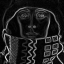
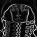
* Summary - Examples of the effect of various derivative algorithms on a noisy version of Figure 30a (SNR = 29 dB) are shown in Figure 31a-c. The effect of various magnitude gradient algorithms on Figure 30a are shown in Figure 32a-c. After processing, all images are contrast stretched as in eq. for display purposes.


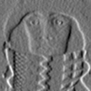
 =1.5) & eq. ii
 Figure 31: Application of various algorithms for hx - the horizontal derivative.
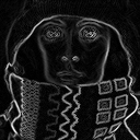
 =1.5) & eq. ii
Figure 32: Various algorithms for the magnitude gradient,
| a|.
a|.
The magnitude gradient takes on large values where there are strong edges in
the image. Appropriate choice of  in the Gaussian-based
derivative (Figure 31c) or gradient (Figure 32c) permits computation of
virtually any of the other forms - simple, Prewitt, Sobel, etc. In that sense,
the Gaussian derivative represents a superset of derivative filters.

where h2x and h2y are second derivative filters. In the frequency domain we have for the Laplacian filter (from eq. ):

The transfer function of a Laplacian corresponds to a parabola (u,v) = -(u2 + v2).
* Basic second derivative filter - This filter is specified by:

and the frequency spectrum of this filter, in each direction, is given by:

over the frequency range - <=
<=  <=
<=  . The two,
one-dimensional filters can be used in the manner suggested by eq. or combined
into one, two-dimensional filter as:

and used as in eq. .
* Frequency domain Laplacian - This filter is the implementation of the general recipe given in eq. and for the Laplacian filter takes the form:

* Gaussian second derivative filter - This is the straightforward
extension of the Gaussian first derivative filter described above and can be
applied independently in each dimension. We first apply Gaussian smoothing with
a  chosen on the basis of the problem specification. We then
apply the desired second derivative filter eq. or eq. . Again there is the
choice among the various Gaussian smoothing algorithms.
For efficiency, we can use the recursive implementation and combine the two steps--smoothing and derivative operation--as follows:

where the various coefficients are defined in eq. . Again, the first (forward) equation is applied from n = 0 up to n = N - 1 while the second (backward) equation is applied from n = N - 1 down to n = 0.
* Alternative Laplacian filters - Again one-dimensional digital filter design techniques offer us powerful methods to create filters that are optimized for a specific problem. Using the Parks-McClellan design algorithm, we can choose the frequency bands where we want the second derivative to be taken and the frequency bands where we want the noise to be suppressed. The algorithm will then produce a real, even filter with a minimum length that meets the specifications.
As an example, if we want a filter that has second derivative characteristics
in a passband (with weight 1.0) in the frequency range 0.0 <=
 <= 0.3
 and a stopband (with weight 3.0) in the range
0.32
 <=
<=  <=
<=  , then the algorithm produces the
following optimized seven sample filter:

The Laplacian can then be calculated as in eq. .
* SDGD filter - A filter that is especially useful in edge finding and object measurement is the Second-Derivative-in-the-Gradient-Direction (SDGD) filter. This filter uses five partial derivatives:

Note that Axy = Ayx which accounts for the five derivatives.
This SDGD combines the different partial derivatives as follows:

As one might expect, the large number of derivatives involved in this filter
implies that noise suppression is important and that Gaussian derivative
filters--both first and second order--are highly recommended if not required .
It is also necessary that the first and second derivative filters have
essentially the same passbands and stopbands. This means that if the first
derivative filter h1x is given by [1 0 -1] (eq. ii)
then the second derivative filter should be given by h1x
 h1x = h2x = [1 0
-2 0 1].
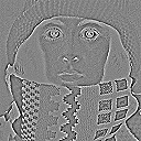
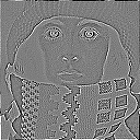
* Summary - The effects of the various second derivative filters are illustrated in Figure 33a-e. All images were contrast stretched for display purposes using eq. and the parameters 1% and 99%.
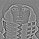
 =1.0) & eq.
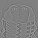
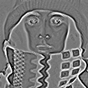 (d) (e) "Designer" - eq. SDGD (
 =1.0) -
eq.
 Figure 33: Various algorithms for the Laplacian and Laplacian-related filters.
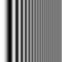
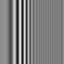

Figure 34: Various convolution algorithms applied to sinusoidal test image.
