


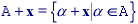
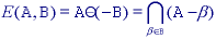
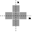
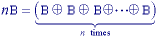
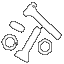
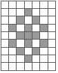
In Section 1 we defined an image as an (amplitude) function of two, real (coordinate) variables a(x,y) or two, discrete variables a[m,n]. An alternative definition of an image can be based on the notion that an image consists of a set (or collection) of either continuous or discrete coordinates. In a sense the set corresponds to the points or pixels that belong to the objects in the image. This is illustrated in Figure 35 which contains two objects or sets A and B. Note that the coordinate system is required. For the moment we will consider the pixel values to be binary as discussed in Section 2.1 and 9.2.1. Further we shall restrict our discussion to discrete space (Z2). More general discussions can be found in .
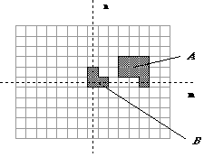
Figure 35: A binary image containing two object sets A and B.
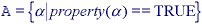
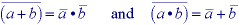
The object A consists of those pixels a that share some common property:
As an example, object B in Figure 35 consists of {[0,0], [1,0], [0,1]}.
The background of A is given by Ac (the complement of A) which is defined as those elements that are not in A:
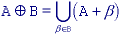
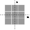
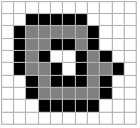
In Figure 3 we introduced the concept of neighborhood connectivity. We now observe that if an object A is defined on the basis of C-connectivity (C=4, 6, or 8) then the background Ac has a connectivity given by 12 - C. The necessity for this is illustrated for the Cartesian grid in Figure 36.
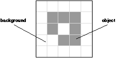
Figure 36: A binary image requiring careful definition of object and background connectivity.
 ,
,  , c} plus
translation:
, c} plus
translation:
* Translation - Given a vector x and a set A, the translation, A + x, is defined as:
Note that, since we are dealing with a digital image composed of pixels at integer coordinate positions (Z2), this implies restrictions on the allowable translation vectors x.
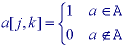
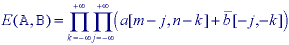
The basic Minkowski set operations--addition and subtraction--can now be defined. First we note that the individual elements that comprise B are not only pixels but also vectors as they have a clear coordinate position with respect to [0,0]. Given two sets A and B:
where
 .
These two operations are illustrated in Figure 37 for the objects defined in
Figure 35.
.
These two operations are illustrated in Figure 37 for the objects defined in
Figure 35.
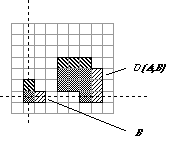
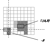 (a) Dilation D(A,B) (b) Erosion
E(A,B)
(a) Dilation D(A,B) (b) Erosion
E(A,B)Figure 37: A binary image containing two object sets A and B. The three pixels in B are "color-coded" as is their effect in the result.
While either set A or B can be thought of as an "image", A is usually considered as the image and B is called a structuring element. The structuring element is to mathematical morphology what the convolution kernel is to linear filter theory.
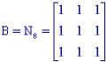
Dilation, in general, causes objects to dilate or grow in size; erosion causes objects to shrink. The amount and the way that they grow or shrink depend upon the choice of the structuring element. Dilating or eroding without specifying the structural element makes no more sense than trying to lowpass filter an image without specifying the filter. The two most common structuring elements (given a Cartesian grid) are the 4-connected and 8-connected sets, N4 and N8. They are illustrated in Figure 38.
 (a) N4 (b)
N8
(a) N4 (b)
N8 Figure 38: The standard structuring elements N4 and N8.
Dilation and erosion have the following properties:


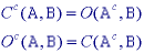
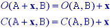
With A as an object and Ac as the background, eq. says that the dilation of an object is equivalent to the erosion of the background. Likewise, the erosion of the object is equivalent to the dilation of the background.
Except for special cases:

Erosion has the following translation property:

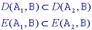
Dilation and erosion have the following important properties. For
any arbitrary structuring element B and two image objects
A1 and A2 such that
A1  A2
(A1 is a proper subset of
A2):
A2
(A1 is a proper subset of
A2):
For two structuring elements B1 and
B2 such that B1
B2:

The decomposition theorems below make it possible to find efficient implementations for morphological filters.


An important decomposition theorem is due to Vincent . First, we require some definitions. A convex set (in R2) is one for which the straight line joining any two points in the set consists of points that are also in the set. Care must obviously be taken when applying this definition to discrete pixels as the concept of a "straight line" must be interpreted appropriately in Z2. A set is bounded if each of its elements has a finite magnitude, in this case distance to the origin of the coordinate system. A set is symmetric if B = -B. The sets N4 and N8 in Figure 38 are examples of convex, bounded, symmetric sets.
Vincent's theorem, when applied to an image consisting of discrete pixels,
states that for a bounded, symmetric structuring element B that
contains no holes and contains its own center,
 :
:

where  A is the contour of the object. That is,
A is the set of pixels that have a background pixel
as a neighbor. The implication of this theorem is that it is not necessary to
process all the pixels in an object in order to compute a dilation or
(using eq. ) an erosion. We only have to process the boundary pixels.
This also holds for all operations that can be derived from dilations
and erosions. The processing of boundary pixels instead of object pixels
means that, except for pathological images, computational complexity can be
reduced from O(N2) to O(N) for an
N x N image. A number of "fast" algorithms can be found
in the literature that are based on this result . The simplest dilation and
erosion algorithms are frequently described as follows.
A is the contour of the object. That is,
A is the set of pixels that have a background pixel
as a neighbor. The implication of this theorem is that it is not necessary to
process all the pixels in an object in order to compute a dilation or
(using eq. ) an erosion. We only have to process the boundary pixels.
This also holds for all operations that can be derived from dilations
and erosions. The processing of boundary pixels instead of object pixels
means that, except for pathological images, computational complexity can be
reduced from O(N2) to O(N) for an
N x N image. A number of "fast" algorithms can be found
in the literature that are based on this result . The simplest dilation and
erosion algorithms are frequently described as follows.
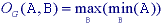
* Dilation - Take each binary object pixel (with value "1") and set all background pixels (with value "0") that are C-connected to that object pixel to the value "1".
* Erosion - Take each binary object pixel (with value "1") that is C-connected to a background pixel and set the object pixel value to "0".
Comparison of these two procedures to eq. where B = NC=4 or NC=8 shows that they are equivalent to the formal definitions for dilation and erosion. The procedure is illustrated for dilation in Figure 39.
 (a) B = N4 (b) B=
N8
(a) B = N4 (b) B=
N8Figure 39: Illustration of dilation. Original object pixels are in gray; pixels added through dilation are in black.
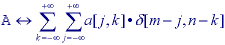
where  and * are the Boolean operations OR and
AND as defined in eqs. (81) and (82), a[j,k] is a
characteristic function that takes on the Boolean values "1" and
"0" as follows:
and * are the Boolean operations OR and
AND as defined in eqs. (81) and (82), a[j,k] is a
characteristic function that takes on the Boolean values "1" and
"0" as follows:
and d[m,n] is a Boolean version of the Dirac delta function that takes on the Boolean values "1" and "0" as follows:
Dilation for binary images can therefore be written as:
which, because Boolean OR and AND are commutative, can also be written as
Using De Morgan's theorem:
on eq. together with eq. , erosion can be written as:
Thus, dilation and erosion on binary images can be viewed as a form of convolution over a Boolean algebra.
In Section 9.3.2 we saw that, when convolution is employed, an appropriate choice of the boundary conditions for an image is essential. Dilation and erosion--being a Boolean convolution--are no exception. The two most common choices are that either everything outside the binary image is "0" or everything outside the binary image is "1".


The opening and closing have the following properties:
For the opening with structuring element B and images
A, A1, and A2,
where A1 is a subimage of A2
(A1  A2):
A2):


For the closing with structuring element B and images
A, A1, and A2,
where A1 is a subimage of A2
(A1 A2):


The two properties given by eqs. and are so important to mathematical morphology that they can be considered as the reason for defining erosion with -B instead of B in eq. .
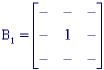
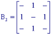
where B1 and B2 are bounded,
disjoint structuring elements. (Note the use of the notation from eq. (81).)
Two sets are disjoint if B1
B2 = ![]() , the
empty set. In an important sense the hit-and-miss
operator is the morphological equivalent of template
matching, a well-known technique for matching patterns based upon
cross-correlation. ere, we have a template B1 for the
object and a template B2 for the background.
, the
empty set. In an important sense the hit-and-miss
operator is the morphological equivalent of template
matching, a well-known technique for matching patterns based upon
cross-correlation. ere, we have a template B1 for the
object and a template B2 for the background.
 (a) (b) (c)
 Figure 40: Structuring elements B, B1, and B2 that are 3 x 3 and symmetric.
The results of processing are shown in Figure 41 where the binary value "1" is shown in black and the value "0" in white.


a) Image A b) Dilation with 2B c) Erosion with 2B


d) Opening with 2B e) Closing with 2B f) it-and-Miss with B1 and B2
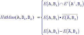
The opening operation can separate objects that are connected in a binary image. The closing operation can fill in small holes. Both operations generate a certain amount of smoothing on an object contour given a "smooth" structuring element. The opening smoothes from the inside of the object contour and the closing smoothes from the outside of the object contour. The hit-and-miss example has found the 4-connected contour pixels. An alternative method to find the contour is simply to use the relation:
or
i) one-pixel thick,
ii) through the "middle" of the object, and,
iii) preserves the topology of the object.
These are not always realizable. Figure 42 shows why this is the case.
 (a) (b)
 Figure 42: Counterexamples to the three requirements.
In the first example, Figure 42a, it is not possible to generate a line that is one pixel thick and in the center of an object while generating a path that reflects the simplicity of the object. In Figure 42b it is not possible to remove a pixel from the 8-connected object and simultaneously preserve the topology--the notion of connectedness--of the object. Nevertheless, there are a variety of techniques that attempt to achieve this goal and to produce a skeleton.
A basic formulation is based on the work of Lantuéjoul . The skeleton subset Sk(A) is defined as:

where K is the largest value of k before the set
Sk(A) becomes empty. (From eq. ,
 ).
The structuring element B is chosen (in Z2) to
approximate a circular disc, that is, convex, bounded and symmetric. The
skeleton is then the union of the skeleton subsets:
).
The structuring element B is chosen (in Z2) to
approximate a circular disc, that is, convex, bounded and symmetric. The
skeleton is then the union of the skeleton subsets:
An elegant side effect of this formulation is that the original object can be reconstructed given knowledge of the skeleton subsets Sk(A), the structuring element B, and K:
This formulation for the skeleton, however, does not preserve the topology, a requirement described in eq. .
An alternative point-of-view is to implement a thinning, an erosion that reduces the thickness of an object without permitting it to vanish. A general thinning algorithm is based on the hit-and-miss operation:

Depending on the choice of B1 and B2, a large variety of thinning algorithms--and through repeated application skeletonizing algorithms--can be implemented.
A quite practical implementation can be described in another way. If we restrict ourselves to a 3 x 3 neighborhood, similar to the structuring element B = N8 in Figure 40a, then we can view the thinning operation as a window that repeatedly scans over the (binary) image and sets the center pixel to "0" under certain conditions. The center pixel is not changed to "0" if and only if:
i) an isolated pixel is found (e.g. Figure 43a),
ii) removing a pixel would change the connectivity (e.g. Figure 43b),
iii) removing a pixel would shorten a line (e.g. Figure 43c).
As pixels are (potentially) removed in each iteration, the process is called a conditional erosion. Three test cases of eq. are illustrated in Figure 43. In general all possible rotations and variations have to be checked. As there are only 512 possible combinations for a 3 x 3 window on a binary image, this can be done easily with the use of a lookup table.


 (a) Isolated pixel (b) Connectivity pixel (c) End pixel
Figure 43: Test conditions for conditional erosion of the center pixel.
If only condition (i) is used then each object will be reduced to a single pixel. This is useful if we wish to count the number of objects in an image. If only condition (ii) is used then holes in the objects will be found. If conditions (i + ii) are used each object will be reduced to either a single pixel if it does not contain a hole or to closed rings if it does contain holes. If conditions (i + ii + iii) are used then the "complete skeleton" will be generated as an approximation to eq. . Illustrations of these various possibilities are given in Figure 44a,b.

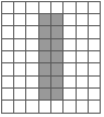
With each iteration the seed image grows (through dilation) but within the set (object) defined by A; S propagates to fill A. The most common choices for B are N4 or N8. Several remarks are central to the use of propagation. First, in a straightforward implementation, as suggested by eq. , the computational costs are extremely high. Each iteration requires O(N2) operations for an N x N image and with the required number of iterations this can lead to a complexity of O(N3). Fortunately, a recursive implementation of the algorithm exists in which one or two passes through the image are usually sufficient, meaning a complexity of O(N2). Second, although we have not paid much attention to the issue of object/background connectivity until now (see Figure 36), it is essential that the connectivity implied by B be matched to the connectivity associated with the boundary definition of A (see eqs. and ). Finally, as mentioned earlier, it is important to make the correct choice ("0" or "1") for the boundary condition of the image. The choice depends upon the application.
Several techniques based upon the use of skeleton and propagation operations in combination with other mathematical morphology operations will be given in Section 10.3.3.


Original = light gray Mask = light gray
 Skeleton = black
Seed = black
Skeleton = black
Seed = black


a) Skeleton with end pixels b) Skeleton without end pixels c) Propagation with N8
Condition eq. i+ii+iii Condition eq. i+ii
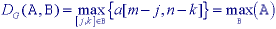
* Gray-level dilation, DG(*), is given by:
For a given output coordinate [m,n], the structuring element is summed with a shifted version of the image and the maximum encountered over all shifts within the J x K domain of B is used as the result. Should the shifting require values of the image A that are outside the M x N domain of A, then a decision must be made as to which model for image extension, as described in Section 9.3.2, should be used.
* Gray-level erosion, EG(*), is given by:
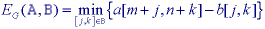
The duality between gray-level erosion and gray-level dilation--the gray-level counterpart of eq. --is somewhat more complex than in the binary case:

where "
 " means that a[j,k] ->
-a[-j,-k].
" means that a[j,k] ->
-a[-j,-k].
The definitions of higher order operations such as gray-level opening and gray-level closing are:


The important properties that were discussed earlier such as idempotence, translation invariance, increasing in A, and so forth are also applicable to gray level morphological processing. The details can be found in Giardina and Dougherty .
In many situations the seeming complexity of gray level morphological
processing is significantly reduced through the use of symmetric structuring
elements where b[j,k] = b[-j,-k]. The
most common of these is based on the use of B = constant =
0. For this important case and using again the domain [j,k]
B, the definitions above reduce to:
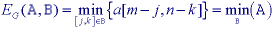
The remarkable conclusion is that the maximum filter and the minimum filter, introduced in Section 9.4.2, are gray-level dilation and gray-level erosion for the specific structuring element given by the shape of the filter window with the gray value "0" inside the window. Examples of these operations on a simple one-dimensional signal are shown in Figure 45.
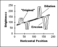
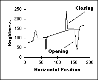
Figure 45: Morphological filtering of gray-level data.
For a rectangular window, J x K, the two-dimensional maximum or minimum filter is separable into two, one-dimensional windows. Further, a one-dimensional maximum or minimum filter can be written in incremental form. (See Section 9.3.2.) This means that gray-level dilations and erosions have a computational complexity per pixel that is O(constant), that is, independent of J and K. (See also Table 13.)
The operations defined above can be used to produce morphological algorithms
for smoothing, gradient determination and a version of the Laplacian. All are
constructed from the primitives for gray-level dilation and
gray-level erosion and in all cases the maximum and
minimum filters are taken over the domain
 .
.
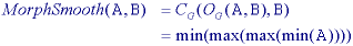
Note that we have suppressed the notation for the structuring element B under the max and min operations to keep the notation simple. Its use, however, is understood.
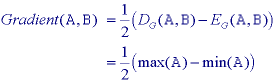
a) Dilation b) Erosion c) Smoothing
 d) Gradient e) Laplacian
 Figure 46: Examples of gray-level morphological filters.