 ), and time (t). Unless otherwise stated, we will
consider the case of 2D, monochromatic, static images in this chapter.


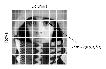
A digital image a[m,n] described in a 2D discrete space is derived from an analog image a(x,y) in a 2D continuous space through a sampling process that is frequently referred to as digitization. The mathematics of that sampling process will be described in Section 5. For now we will look at some basic definitions associated with the digital image. The effect of digitization is shown in Figure 1.
The 2D continuous image a(x,y) is divided into N
rows and M columns. The intersection of a row and a column
is termed a pixel. The value assigned to the integer coordinates
[m,n] with {m=0,1,2,...,M-1} and
{n=0,1,2,...,N-1} is a[m,n]. In fact, in
most cases a(x,y)--which we might consider to be the
physical signal that impinges on the face of a 2D sensor--is actually a
function of many variables including depth (z), color
( ), and time (t). Unless otherwise stated, we will
consider the case of 2D, monochromatic, static images in this chapter.

Figure 1: Digitization of a continuous image. The pixel at coordinates [m=10, n=3] has the integer brightness value 110.
The image shown in Figure 1 has been divided into N = 16 rows and M = 16 columns. The value assigned to every pixel is the average brightness in the pixel rounded to the nearest integer value. The process of representing the amplitude of the 2D signal at a given coordinate as an integer value with L different gray levels is usually referred to as amplitude quantization or simply quantization.

