


The method by which images are produced--the interaction between objects in real space, the illumination, and the camera--frequently leads to situations where the image exhibits significant shading across the field-of-view. In some cases the image might be bright in the center and decrease in brightness as one goes to the edge of the field-of-view. In other cases the image might be darker on the left side and lighter on the right side. The shading might be caused by non-uniform illumination, non-uniform camera sensitivity, or even dirt and dust on glass (lens) surfaces. In general this shading effect is undesirable. Eliminating it is frequently necessary for subsequent processing and especially when image analysis or image understanding is the final goal.

with the object representing various imaging modalities such as:
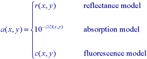
where at position (x,y), r(x,y) is the reflectance, OD(x,y) is the optical density, and c(x,y) is the concentration of fluorescent material. Parenthetically, we note that the fluorescence model only holds for low concentrations. The camera may then contribute gain and offset terms, as in eq. (74), so that:

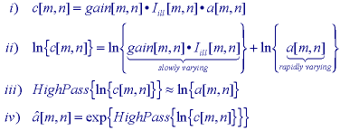
In general we assume that Iill[m,n] is slowly varying compared to a[m,n].
* A posteriori estimate - In this case we attempt to extract the shading estimate from c[m,n]. The most common possibilities are the following.
Lowpass filtering - We compute a smoothed version of c[m,n] where the smoothing is large compared to the size of the objects in the image. This smoothed version is intended to be an estimate of the background of the image. We then subtract the smoothed version from c[m,n] and then restore the desired DC value. In formula:

where
 is the estimate of a[m,n]. Choosing the appropriate
lowpass filter means knowing the appropriate spatial frequencies in the Fourier
domain where the shading terms dominate.
omomorphic filtering - We note that, if the offset[m,n] = 0, then c[m,n] consists solely of multiplicative terms. Further, the term {gain[m,n]*Iill[m,n]} is slowly varying while a[m,n] presumably is not. We therefore take the logarithm of c[m,n] to produce two terms one of which is low frequency and one of which is high frequency. We suppress the shading by high pass filtering the logarithm of c[m,n] and then take the exponent (inverse logarithm) to restore the image. This procedure is based on homomorphic filtering as developed by Oppenheim, Schafer and Stockham . In formula:
Morphological filtering - We again compute a smoothed version of c[m,n] where the smoothing is large compared to the size of the objects in the image but this time using morphological smoothing as in eq. . This smoothed version is the estimate of the background of the image. We then subtract the smoothed version from c[m,n] and then restore the desired DC value. In formula:

Choosing the appropriate morphological filter window means knowing (or estimating) the size of the largest objects of interest.
* A priori estimate - If it is possible to record test (calibration) images through the cameras system, then the most appropriate technique for the removal of shading effects is to record two images - BLACK[m,n] and WHITE[m,n]. The BLACK image is generated by covering the lens leading to b[m,n] = 0 which in turn leads to BLACK[m,n] = offset[m,n]. The WHITE image is generated by using a[m,n] = 1 which gives WHITE[m,n] = gain[m,n]*Iill[m,n] + offset[m,n]. The correction then becomes:

The constant term is chosen to produce the desired dynamic range.
The effects of these various techniques on the data from Figure 45 are shown in Figure 47. The shading is a simple, linear ramp increasing from left to right; the objects consist of Gaussian peaks of varying widths.
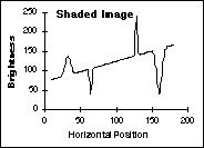 (a) Original
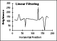
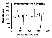
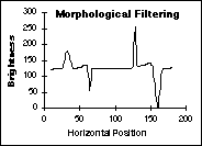
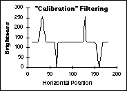
Figure 47: Comparison of various shading correction algorithms. The final result (d) is identical to the original (not shown).
In summary, if it is possible to obtain BLACK and WHITE calibration images, then eq. is to be preferred. If this is not possible, then one of the other algorithms will be necessary.
